
AINode
AINode
AINode is a native IoTDB node that supports the registration, management, and invocation of time series related models. It includes industry-leading self-developed time series large models, such as the Timer series models developed by Tsinghua University. Models can be invoked using standard SQL statements, enabling millisecond-level real-time inference on time series data, and supporting application scenarios such as time series trend prediction, missing value filling, and anomaly value detection.
The system architecture is shown in the following figure:
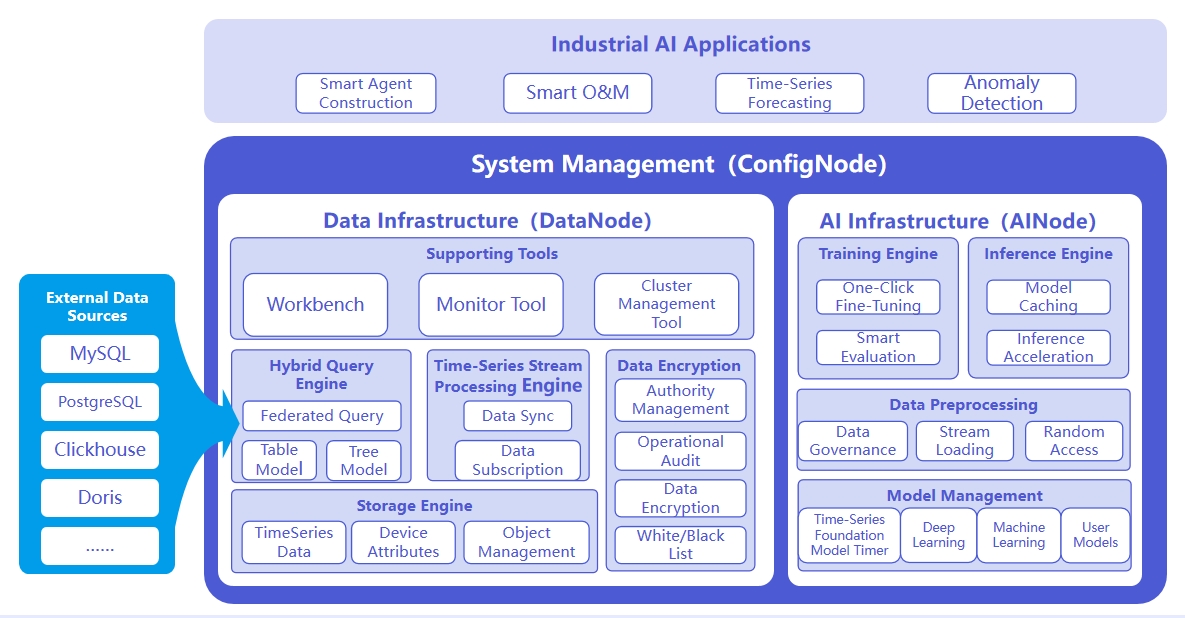
The responsibilities of the three nodes are as follows:
- ConfigNode: Responsible for distributed node management and load balancing.
- DataNode: Responsible for receiving and parsing user SQL requests; responsible for storing time series data; responsible for data preprocessing calculations.
- AINode: Responsible for managing and using time series models.
1. Advantages and Features
Compared to building a machine learning service separately, it has the following advantages:
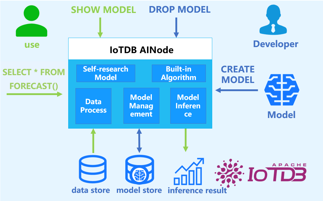
- Simple and Easy to Use: No need to use Python or Java programming, you can complete the entire process of machine learning model management and inference using SQL statements. For example, creating a model can be done using the CREATE MODEL statement, and using a model for inference can be done using the
SELECT * FROM FORECAST (...)statement, making it more simple and convenient. - Avoid Data Migration: Using IoTDB-native machine learning can directly apply data stored in IoTDB to machine learning model inference without moving data to a separate machine learning service platform, thus accelerating data processing, improving security, and reducing costs.

- Built-in Advanced Algorithms: Supports industry-leading machine learning analysis algorithms, covering typical time series analysis tasks, and empowering time series databases with native data analysis capabilities. For example:
- Time Series Forecasting: Learning change patterns from past time series data; outputting the most likely predictions for future sequences based on given past observations.
- Time Series Anomaly Detection: Detecting and identifying abnormal values in given time series data to help discover abnormal behavior in time series.
2. Basic Concepts
- Model (Model): A machine learning model that takes time series data as input and outputs the results or decisions of the analysis task. The model is the basic management unit of AINode, supporting the creation (registration), deletion, query, modification (fine-tuning), and use (inference) of models.
- Create (Create): Load the external designed or trained model file or algorithm into AINode, managed and used uniformly by IoTDB.
- Inference (Inference): Use the created model to complete the time series analysis task on the specified time series data.
- Built-in (Built-in): AINode comes with common time series analysis scenario (e.g., prediction and anomaly detection) machine learning algorithms or self-developed models.
3. Installation and Deployment
AINode deployment can be referred to the documentation AINode Deployment.
4. Usage Guide
TimechoDB-AINode supports three major functions: model inference, model fine-tuning, and model management (registration, viewing, deletion, loading, unloading, etc.). The following sections will provide detailed explanations.
4.1 Model Inference
The AINode table model supports two major inference capabilities: time series prediction and time series classification.
4.1.1 Time Series Prediction
The time series prediction capability provided by the AINode table model includes:
- Univariate Prediction: Supports prediction of a single target variable.
- Covariate Prediction: Can simultaneously predict multiple target variables and supports introducing covariates in prediction to improve accuracy.
The following sections will detail the syntax definition, parameter descriptions, and usage examples of the prediction inference function.
- SQL Syntax
SELECT * FROM FORECAST(
   MODEL_ID,
   TARGETS, -- SQL to get target variables
   [HISTORY_COVS, -- String, SQL to get historical covariates
   FUTURE_COVS, -- String, SQL to get future covariates
   STATIC_COVS, -- Supported from V2.0.10.2. String, SQL to get static covariates. It must return a single row; SELECT DISTINCT is recommended.
   OUTPUT_START_TIME,
   OUTPUT_LENGTH,
   OUTPUT_INTERVAL,
   TIMECOL,
   PRESERVE_INPUT,
   AUTO_ADAPT, -- Boolean type, indicating whether adaptive mode is enabled.
   MODEL_OPTIONS]?
)- Built-in model inference does not require a registration process. By using the forecast function and specifying model_id, you can use the inference function of the model.
- Parameter description
| Parameter Name | Parameter Type | Parameter Attributes | Description | Required | Notes |
|---|---|---|---|---|---|
| model_id | Scalar parameter | String type | Unique identifier of the prediction model | Yes | |
| targets | Table parameter | SET SEMANTIC | Input data for the target variables to be predicted. IoTDB will automatically sort the data in ascending order of time before passing it to AINode. | Yes | Use SQL to describe the input data with target variables. If the input SQL is invalid, corresponding query errors will be reported. |
| history_covs | Scalar parameter | String type (valid table model query SQL), default: none | Specifies historical data of covariates for this prediction task, which are used to assist in predicting target variables. AINode will not output prediction results for historical covariates. Before passing data to the model, AINode will automatically sort the data in ascending order of time. | No | 1. All timestamps of the historical covariate data must be equal to all timestamps of the target variables; 2. Query results can only contain FIELD columns; 3. Other: Different models may have specific requirements, and errors will be thrown if not met. |
| future_covs | Scalar parameter | String type (valid table model query SQL), default: none | Specifies future data of some covariates for this prediction task, which are used to assist in predicting target variables. Before passing data to the model, AINode will automatically sort the data in ascending order of time. | No | 1. Can only be specified when history_covs is set; 2. The covariate names involved must be a subset of history_covs; 3. Query results can only contain FIELD columns; 4. Other: Different models may have specific requirements, and errors will be thrown if not met. |
| static_covs | Scalar parameter | String (valid table model query SQL), default: empty string | Supported from V2.0.10.2. Specifies the SQL used to fetch static covariates. Usually, use SELECT DISTINCT on ATTRIBUTE columns. Each static covariate remains constant over the entire sequence. AINode takes its single value into the inference pipeline and does not output prediction results for it. Numeric types and categorical type STRING are supported. | No | 1. The SQL must return exactly one row; otherwise, an error is reported. 2. The SQL must not contain the time column; otherwise, an error is reported. 3. If this parameter is specified but no data is found, an error is reported. 4. For models without a static covariate channel, the static covariates are ignored after a warning is logged, and no error is reported. Currently, none of the built-in models has this channel. |
| output_start_time | Scalar parameter | Timestamp type. Default value: last timestamp of target variable + output_interval | Starting timestamp of output prediction points [i.e., forecast start time] | No | Must be greater than the maximum timestamp of target variable timestamps |
| output_length | Scalar parameter | INT32 type. Default value: 96 | Output window size | No | Must be greater than 0 |
| output_interval | Scalar parameter | Time interval type. Default value: (last timestamp - first timestamp of input data) / n - 1 | Time interval between output prediction points. Supported units: ns, us, ms, s, m, h, d, w | No | Must be greater than 0 |
| timecol | Scalar parameter | String type. Default value: time | Name of time column | No | Must be a TIMESTAMP column existing in targets |
| preserve_input | Scalar parameter | Boolean type. Default value: false | Whether to retain all original rows of target variable input in the output result set | No | |
| auto_adapt | Scalar parameter | Boolean type, default value: true | Whether to enable adaptive processing for covariate inference. | No | When adaptive mode is enabled: 1. If the set of future covariates ( future_covs) is not a subset of the historical covariates (history_covs), any future covariates not present in the historical set will be automatically discarded.2. If the length of any historical covariate does not match the length of the input target variable: a. If shorter, pad zeros at the beginning; b. If longer, discard the earliest data points. 3. If the length of any future covariate does not match the prediction length ( output_length): a. If shorter, pad zeros at the end; b. If longer, discard the most recent data points. |
| model_options | Scalar parameter | String type. Default value: empty string | Key-value pairs related to the model, such as whether to normalize the input. Different key-value pairs are separated by ';'. | No |
Notes:
- Default behavior: Predict all columns of targets. Currently, only supports INT32, INT64, FLOAT, DOUBLE types.
- Input data requirements:
- Must contain a time column.
- Row count requirements: If insufficient, an error will be reported; if exceeding the maximum, the last data will be automatically truncated.
- Column count requirements: Univariate models only support single columns, multi-column will report errors; covariate models usually have no restrictions unless the model itself has clear constraints.
- For covariate prediction, the SQL statement must explicitly specify the DATABASE.
- Static covariate-specific constraints:
- Single-row constraint: The SQL must return exactly one row. Each static covariate corresponds to a constant value, usually obtained by querying ATTRIBUTE columns with SELECT DISTINCT.
- No time column: Static covariates are independent of time, so the SQL must not contain the time column.
- Supported types: STRING (categorical) and numeric types (INT32/INT64/FLOAT/DOUBLE) are allowed.
- Model adaptation: If a model without this channel uses static covariates, the static covariates are ignored after a warning is logged, and no error is reported. Currently, none of the built-in models has this channel.
- Output results:
- Includes all target variable columns, with data types consistent with the original table.
- If
preserve_input=trueis specified, an additionalis_inputcolumn will be added to identify original data rows. - Static covariates are used only as auxiliary input information and are not output as prediction results, so they do not appear in the result set.
- Timestamp generation:
- Uses
OUTPUT_START_TIME(optional) as the starting time point for prediction and divides historical and future data. - Uses
OUTPUT_INTERVAL(optional, default is the sampling interval of input data) as the output time interval. The timestamp of the Nth row is calculated as:OUTPUT_START_TIME + (N - 1) * OUTPUT_INTERVAL.
- Uses
- Usage Examples
Example 1: Univariate Prediction
Create database etth and table eg in advance
create database etth;
create table eg (hufl FLOAT FIELD, hull FLOAT FIELD, mufl FLOAT FIELD, mull FLOAT FIELD, lufl FLOAT FIELD, lull FLOAT FIELD, ot FLOAT FIELD)
Prepare original data ETTh1-tab.
You can import the raw data using the import-data script. For example:
./tools/import-data.sh -ft csv -sql_dialect table -db etth -table eg -s ~/Desktop/model-compare-html/ETTh1-tab.csvUse the first 96 rows of data from column ot in table eg to predict its future 1440 rows of data.
IoTDB:etth> select Time, HUFL,HULL,MUFL,MULL,LUFL,LULL,OT from eg LIMIT 1440
+-----------------------------+------+-----+-----+-----+-----+-----+------+
|                         Time|  HUFL| HULL| MUFL| MULL| LUFL| LULL|    OT|
+-----------------------------+------+-----+-----+-----+-----+-----+------+
|2016-07-01T00:00:00.000+08:00| 5.827|2.009|1.599|0.462|4.203| 1.34|30.531|
|2016-07-01T01:00:00.000+08:00| 5.693|2.076|1.492|0.426|4.142|1.371|27.787|
|2016-07-01T02:00:00.000+08:00| 5.157|1.741|1.279|0.355|3.777|1.218|27.787|
|2016-07-01T03:00:00.000+08:00|  5.09|1.942|1.279|0.391|3.807|1.279|25.044|
......
Total line number = 1440
It costs 0.119s

IoTDB:etth> select * from forecast(
     model_id => 'sundial',
     targets => (select Time, ot from etth.eg where time >= 2016-08-07T18:00:00.000+08:00 limit 1440) order BY time,
     output_length => 96
)
+-----------------------------+---------+
|                         time|       ot|
+-----------------------------+---------+
|2016-10-06T18:00:00.000+08:00|20.733124|
|2016-10-06T19:00:00.000+08:00|20.258146|
|2016-10-06T20:00:00.000+08:00|20.022043|
|2016-10-06T21:00:00.000+08:00|19.789446|
......
Total line number = 96
It costs 1.615s
Example 2: Covariate Prediction
Create table tab_real (to store original real data) in advance
create table tab_real (target1 DOUBLE FIELD, target2 DOUBLE FIELD, cov1 DOUBLE FIELD, cov2 DOUBLE FIELD, cov3 DOUBLE FIELD);Prepare original data
-- Insert statement
IoTDB:etth> INSERT INTO tab_real (time, target1, target2, cov1, cov2, cov3) VALUES
(1, 1.0, 1.0, 1.0, 1.0, 1.0),
(2, 2.0, 2.0, 2.0, 2.0, 2.0),
(3, 3.0, 3.0, 3.0, 3.0, 3.0),
(4, 4.0, 4.0, 4.0, 4.0, 4.0),
(5, 5.0, 5.0, 5.0, 5.0, 5.0),
(6, 6.0, 6.0, 6.0, 6.0, 6.0),
(7, NULL, NULL, NULL, NULL, 7.0),
(8, NULL, NULL, NULL, NULL, 8.0);

IoTDB:etth> SELECT * FROM tab_real
+-----------------------------+-------+-------+----+----+----+
|                         time|target1|target2|cov1|cov2|cov3|
+-----------------------------+-------+-------+----+----+----+
|1970-01-01T08:00:00.001+08:00|    1.0|    1.0| 1.0| 1.0| 1.0|
|1970-01-01T08:00:00.002+08:00|    2.0|    2.0| 2.0| 2.0| 2.0|
|1970-01-01T08:00:00.003+08:00|    3.0|    3.0| 3.0| 3.0| 3.0|
|1970-01-01T08:00:00.004+08:00|    4.0|    4.0| 4.0| 4.0| 4.0|
|1970-01-01T08:00:00.005+08:00|    5.0|    5.0| 5.0| 5.0| 5.0|
|1970-01-01T08:00:00.006+08:00|    6.0|    6.0| 6.0| 6.0| 6.0|
|1970-01-01T08:00:00.007+08:00|   null|   null|null|null| 7.0|
|1970-01-01T08:00:00.008+08:00|   null|   null|null|null| 8.0|
+-----------------------------+-------+-------+----+----+----+
Prediction task 1: Use historical covariates cov1, cov2, and cov3 to assist in predicting target variables target1 and target2.
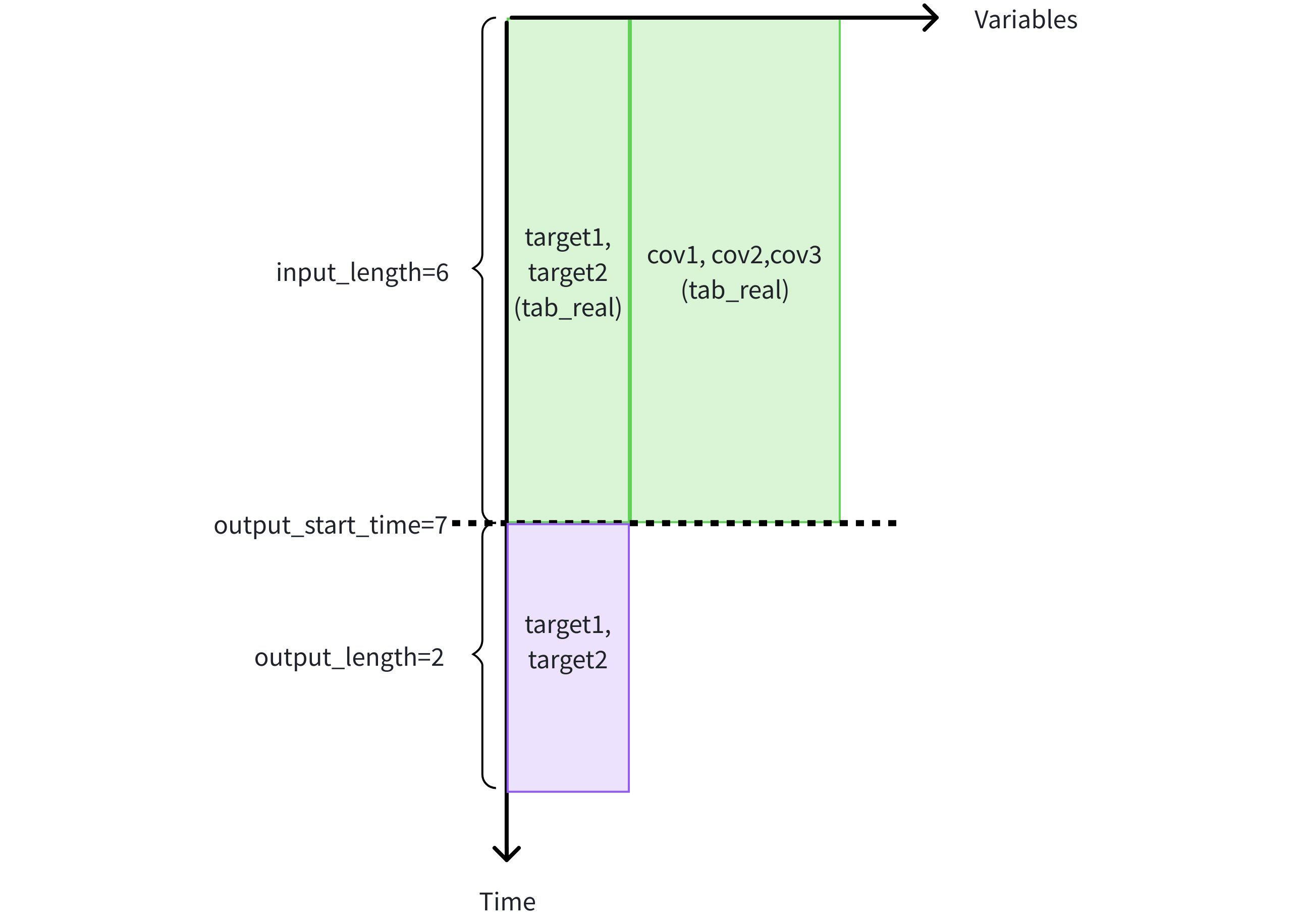
- Use the first 6 rows of historical data from cov1, cov2, cov3, target1, target2 in table tab_real to predict the next 2 rows of target variables target1 and target2.
IoTDB:etth> SELECT * FROM FORECAST (
    MODEL_ID => 'chronos2',
    TARGETS => (
        SELECT TIME, target1, target2
        FROM etth.tab_real
        WHERE TIME < 7
        ORDER BY TIME DESC
        LIMIT 6) ORDER BY TIME,
    HISTORY_COVS => '
        SELECT TIME, cov1, cov2, cov3
        FROM etth.tab_real
        WHERE TIME < 7
        ORDER BY TIME DESC
        LIMIT 6',
    OUTPUT_LENGTH => 2
)
+-----------------------------+-----------------+-----------------+
|                         time|          target1|          target2|
+-----------------------------+-----------------+-----------------+
|1970-01-01T08:00:00.007+08:00|7.338330268859863|7.338330268859863|
|1970-01-01T08:00:00.008+08:00| 8.02529525756836| 8.02529525756836|
+-----------------------------+-----------------+-----------------+
Total line number = 2
It costs 0.315s
- Use the first 6 rows of historical data from cov1, cov2, cov3, target1, target2 in table tab_real to predict the next 2 rows of target variables target1 and target2.
Prediction task 2: Use historical covariates cov1, cov2 and known covariates cov3 in the same table to assist in predicting target variables target1 and target2.
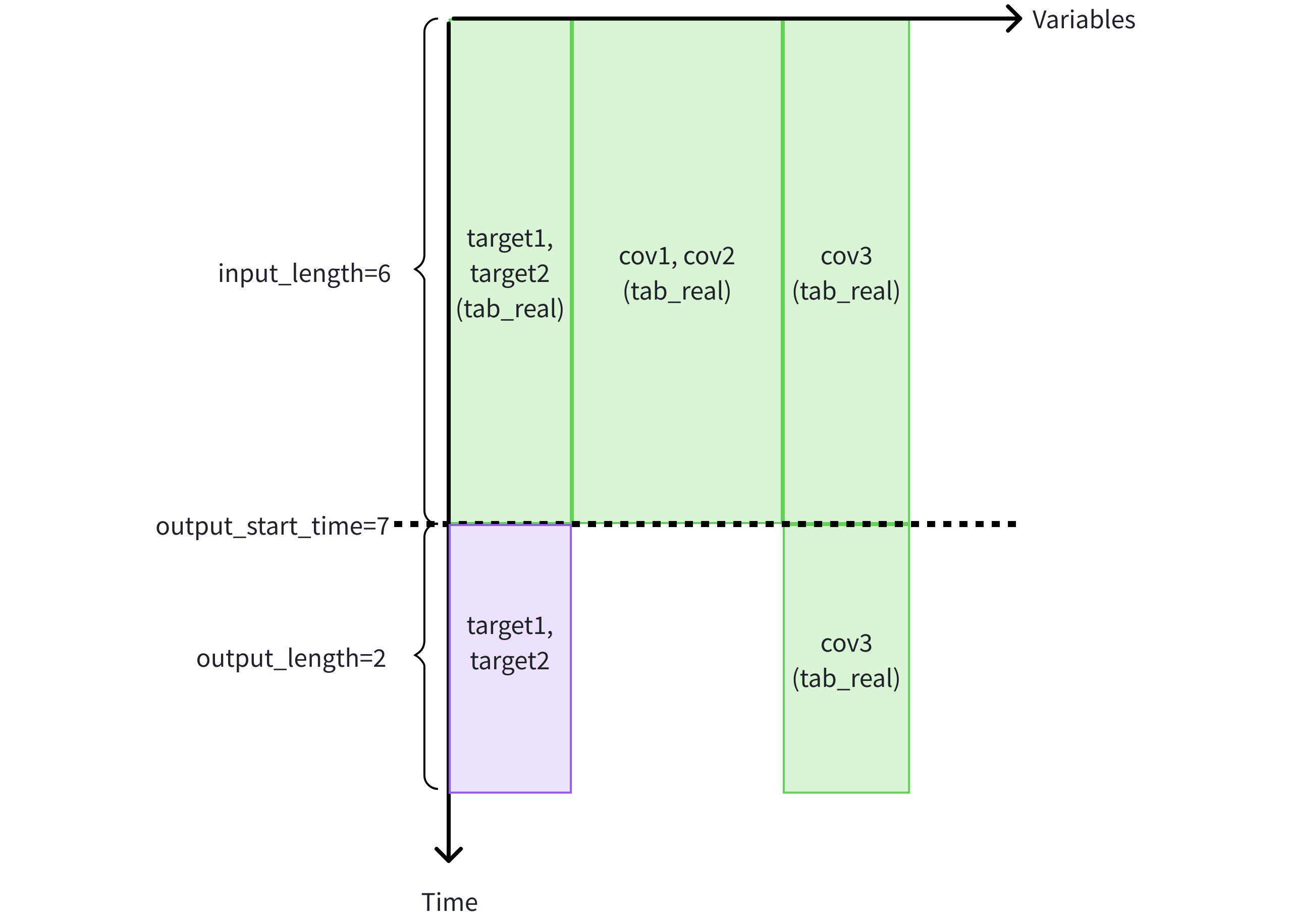
- Use the first 6 rows of historical data from cov1, cov2, cov3, target1, target2 in table tab_real, and known covariate cov3 in the future 2 rows of the same table to predict the next 2 rows of target variables target1 and target2.
IoTDB:etth> SELECT * FROM FORECAST (
    MODEL_ID => 'chronos2',
    TARGETS => (
        SELECT TIME, target1, target2
        FROM etth.tab_real
        WHERE TIME < 7
        ORDER BY TIME DESC
        LIMIT 6) ORDER BY TIME,
    HISTORY_COVS => '
        SELECT TIME, cov1, cov2, cov3
        FROM etth.tab_real
        WHERE TIME < 7
        ORDER BY TIME DESC
        LIMIT 6',
    FUTURE_COVS => '
        SELECT TIME, cov3
        FROM etth.tab_real
        WHERE TIME >= 7
        LIMIT 2',
    OUTPUT_LENGTH => 2
)
+-----------------------------+-----------------+-----------------+
|                         time|          target1|          target2|
+-----------------------------+-----------------+-----------------+
|1970-01-01T08:00:00.007+08:00|7.244050025939941|7.244050025939941|
|1970-01-01T08:00:00.008+08:00|7.907227516174316|7.907227516174316|
+-----------------------------+-----------------+-----------------+
Total line number = 2
It costs 0.291s
- Use the first 6 rows of historical data from cov1, cov2, cov3, target1, target2 in table tab_real, and known covariate cov3 in the future 2 rows of the same table to predict the next 2 rows of target variables target1 and target2.
Prediction task 3: Use historical covariates cov1, cov2 from different tables and known covariates cov3 to assist in predicting target variables target1 and target2.
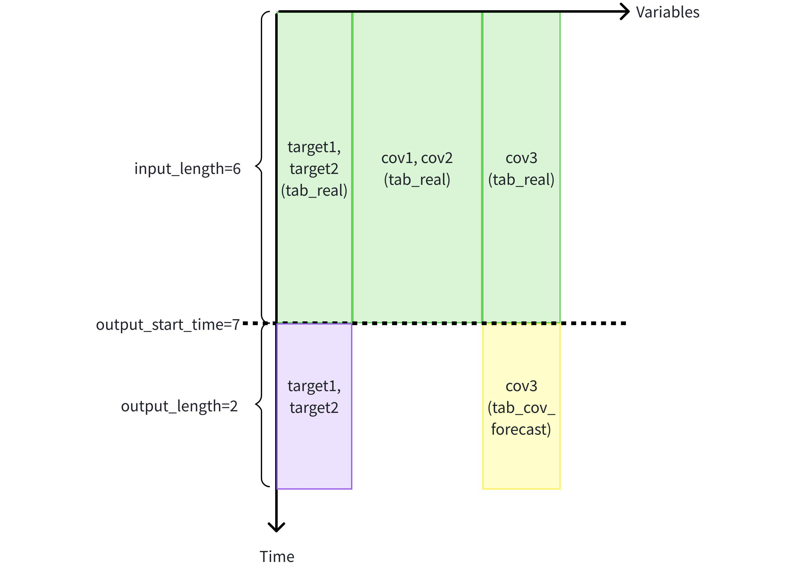
- Create table tab_cov_forecast (to store known covariate cov3 prediction values) in advance, and prepare related data.
create table tab_cov_forecast (cov3 DOUBLE FIELD); -- Insert statement INSERT INTO tab_cov_forecast (time, cov3) VALUES (7, 7.0),(8, 8.0); IoTDB:etth> SELECT * FROM tab_cov_forecast +----+----+ |time|cov3| +----+----+ | 7| 7.0| | 8| 8.0| +----+----+ - Use the first 6 rows of known data from cov1, cov2, cov3, target1, target2 in table tab_real, and known covariate cov3 in the future 2 rows from table tab_cov_forecast to predict the next 2 rows of target variables target1 and target2.
IoTDB:etth> SELECT * FROM FORECAST (
    MODEL_ID => 'chronos2',
    TARGETS => (
        SELECT TIME, target1, target2
        FROM etth.tab_real
        WHERE TIME < 7
        ORDER BY TIME DESC
        LIMIT 6) ORDER BY TIME,
    HISTORY_COVS => '
        SELECT TIME, cov1, cov2, cov3
        FROM etth.tab_real
        WHERE TIME < 7
        ORDER BY TIME DESC
        LIMIT 6',
    FUTURE_COVS => '
        SELECT TIME, cov3
        FROM etth.tab_cov_forecast
        WHERE TIME >= 7
        LIMIT 2',
    OUTPUT_LENGTH => 2
)
+-----------------------------+-----------------+-----------------+
|                         time|          target1|          target2|
+-----------------------------+-----------------+-----------------+
|1970-01-01T08:00:00.007+08:00|7.244050025939941|7.244050025939941|
|1970-01-01T08:00:00.008+08:00|7.907227516174316|7.907227516174316|
+-----------------------------+-----------------+-----------------+
Total line number = 2
It costs 0.351s
- Create table tab_cov_forecast (to store known covariate cov3 prediction values) in advance, and prepare related data.
Prediction task 4: Prediction with static covariate input. chronos2 uses dynamic covariates and ignores static covariates after logging a warning.
- Add two attribute columns, static1 (static covariate 1) and static2 (static covariate 2), to table tab_real, and insert data.
ALTER TABLE tab_real ADD COLUMN IF NOT EXISTS static1 STRING ATTRIBUTE COMMENT 'static covariate 1'; ALTER TABLE tab_real ADD COLUMN IF NOT EXISTS static2 STRING ATTRIBUTE COMMENT 'static covariate 2'; UPDATE tab_real SET static1 = 'one', static2 = 'two'; - Use the first 6 rows of historical data from cov1, cov2, cov3, target1, and target2 in table tab_real, the known future 2 rows of covariate cov3 in the same table, and static covariates static1 and static2 to assist in predicting the next 2 rows of target variables target1 and target2.
IoTDB:etth> SELECT * FROM FORECAST (
    MODEL_ID => 'chronos2',
    TARGETS => (
        SELECT TIME, target1, target2
        FROM etth.tab_real
        WHERE TIME < 7
        ORDER BY TIME DESC
        LIMIT 6) ORDER BY TIME,
    HISTORY_COVS => '
        SELECT TIME, cov1, cov2, cov3
        FROM etth.tab_real
        WHERE TIME < 7
        ORDER BY TIME DESC
        LIMIT 6',
    FUTURE_COVS => '
        SELECT TIME, cov3
        FROM etth.tab_real
        WHERE TIME >= 7
        LIMIT 2',
    STATIC_COVS => '
        SELECT DISTINCT static1, static2
        FROM etth.tab_real',
    OUTPUT_LENGTH => 2
)
+-----------------------------+-----------------+-----------------+
|                         time|          target1|          target2|
+-----------------------------+-----------------+-----------------+
|1970-01-01T08:00:00.007+08:00|7.244050025939941|7.244050025939941|
|1970-01-01T08:00:00.008+08:00|7.907227516174316|7.907227516174316|
+-----------------------------+-----------------+-----------------+
Total line number = 2
It costs 0.291s
- Add two attribute columns, static1 (static covariate 1) and static2 (static covariate 2), to table tab_real, and insert data.
4.1.2 Time Series Classification
Time series classification is a critical capability beyond time series prediction, with extensive applications in industrial scenarios. Its typical paradigm is to input the recent sampling values of multiple measuring points, comprehensively judge the overall operating status of the equipment, and output a classification label for the current status. For example, it can be used for operating status classification of new energy battery pack equipment and other scenarios.
The AINode table model supports executing time series classification tasks by calling covariate classification models.
Note: This feature is available starting from version V2.0.9.1.
- SQL Syntax
SELECT * FROM CLASSIFY(
   MODEL_ID,
   INPUTS -- SQL to retrieve input variables
   [TIMECOL,
   MODEL_OPTIONS]?
)- Parameter Description
| Parameter Name | Parameter Type | Parameter Attribute | Description | Required | Remarks |
|---|---|---|---|---|---|
| model_id | Scalar Parameter | String | Unique identifier of the model used for classification | Yes | - |
| inputs | Table Parameter | SET SEMANTIC | Input data to be classified. IoTDB will automatically sort the data in ascending chronological order before passing it to AINode. | Yes | Describes the input data to be classified via SQL; corresponding query errors will be thrown if the input SQL is invalid. |
| timecol | Scalar Parameter | String, Default: time | Name of the time column | No | Must be a column of TIMESTAMP type present in the inputs result set; otherwise, an error will be thrown. |
| model_options | Scalar Parameter | String, Default: Empty string | Model-related key-value pairs (e.g., whether input normalization is required). Different key-value pairs are separated by ;. | No | Unsupported parameters for a specific model will be ignored without throwing errors. |
Specifications
Input Data Requirements
- Type Constraint: Only INT32, INT64, FLOAT, and DOUBLE data types are supported currently.
- Row Count Constraint: Varies by model. Errors will be thrown if the row count is below the minimum or above the maximum required by the model.
- Column Count Constraint**: Must include a time column. Univariate classification models support only one data column and will throw an error for multiple columns; multivariate classification models generally have no restrictions unless explicitly specified by the model itself.
- Order Constraint: Multivariate zero-shot classification models generally have no order restrictions unless explicitly specified by the model itself.
Output Result
The returned result is a table composed of time series data classification results, and its schema depends on the specific implementation of the model.
- Usage Example
Suppose a project has 10 time series variables with an input length of 192. The custom mantis_custom model is used as an example for time series classification inference.
- Model Registration
CREATE MODEL mantis_custom USING URI 'file:///path/to/mantis'For detailed steps to register a custom model, refer to Section 4.3.
- Execute SQL
IoTDB:etth> SELECT * FROM CLASSIFY (
    MODEL_ID => 'mantis_custom',
    INPUTS => (
        SELECT Time, HUFL,HULL,MUFL,MULL,LUFL,LULL,OT,UT,MT,LT
        FROM eg
        WHERE TIME < 2016-07-09 00:00:00
        ORDER BY TIME DESC
        LIMIT 192) ORDER BY TIME
)- Execution Result
+--------+
|category|
+--------+
|       4|
+--------+
4.2 Model Fine-Tuning
AINode supports model fine-tuning through SQL.
SQL Syntax
createModelStatement
    | CREATE MODEL modelId=identifier (WITH HYPERPARAMETERS '(' hparamPair (',' hparamPair)* ')')? FROM MODEL existingModelId=identifier ON DATASET '(' targetData=string ')'
    ;
hparamPair
    : hparamKey=identifier '=' hyparamValue=primaryExpression
    ;
Parameter Description
| Name | Description |
|---|---|
| modelId | Unique identifier of the fine-tuned model |
| hparamPair | Hyperparameter key-value pairs used for fine-tuning, currently supports the following: train_epochs: int type, number of fine-tuning epochs iter_per_epoch: int type, number of iterations per epoch learning_rate: double type, learning rate |
| existingModelId | Base model used for fine-tuning |
| targetData | SQL to get the dataset used for fine-tuning |
Example
- Select data from the ot field in the specified time range as the fine-tuning dataset, and create the model sundialv3 based on sundial.
IoTDB> set sql_dialect=table
Msg: The statement is executed successfully.
IoTDB> CREATE MODEL sundialv3 FROM MODEL sundial ON DATASET ('SELECT time, ot from etth.eg where 1467302400000 <= time and time < 1517468400001')
Msg: The statement is executed successfully.
IoTDB> show models
+---------------------+---------+-----------+---------+
|              ModelId|ModelType|   Category|    State|
+---------------------+---------+-----------+---------+
|                arima|   sktime|    builtin|   active|
|          holtwinters|   sktime|    builtin|   active|
|exponential_smoothing|   sktime|    builtin|   active|
|     naive_forecaster|   sktime|    builtin|   active|
|       stl_forecaster|   sktime|    builtin|   active|
|         gaussian_hmm|   sktime|    builtin|   active|
|              gmm_hmm|   sktime|    builtin|   active|
|                stray|   sktime|    builtin|   active|
|             timer_xl|    timer|    builtin|   active|
|              sundial|  sundial|    builtin|   active|
|             chronos2|       t5|    builtin|   active|
|            sundialv2|  sundial| fine_tuned|   active|
|            sundialv3|  sundial| fine_tuned| training|
+---------------------+---------+-----------+---------+- Fine-tuning tasks are started asynchronously in the background, which can be seen in the AINode process log; after fine-tuning is completed, query and use the new model.
IoTDB> show models
+---------------------+---------+-----------+---------+
|              ModelId|ModelType|   Category|    State|
+---------------------+---------+-----------+---------+
|                arima|   sktime|    builtin|   active|
|          holtwinters|   sktime|    builtin|   active|
|exponential_smoothing|   sktime|    builtin|   active|
|     naive_forecaster|   sktime|    builtin|   active|
|       stl_forecaster|   sktime|    builtin|   active|
|         gaussian_hmm|   sktime|    builtin|   active|
|              gmm_hmm|   sktime|    builtin|   active|
|                stray|   sktime|    builtin|   active|
|             timer_xl|    timer|    builtin|   active|
|              sundial|  sundial|    builtin|   active|
|             chronos2|       t5|    builtin|   active|
|            sundialv2|  sundial| fine_tuned|   active|
|            sundialv3|  sundial| fine_tuned|   active|
+---------------------+---------+-----------+---------+
4.3 Register Custom Models
The following Transformers models can be registered to AINode:
AINode currently uses transformers version 4.56.2, so when building the model, avoid inheriting interfaces from lower versions (<4.50);
The model must inherit a pipeline for inference tasks of AINode (currently supports prediction pipeline):
- iotdb-core/ainode/iotdb/ainode/core/inference/pipeline/basic_pipeline.py
Before V2.0.9.3
class BasicPipeline(ABC):
    def __init__(self, model_id, **model_kwargs):
        self.model_info = model_info
        self.device = model_kwargs.get("device", "cpu")
        self.model = load_model(model_info, device_map=self.device, **model_kwargs)

    @abstractmethod
    def preprocess(self, inputs, **infer_kwargs):
        """
        Preprocess the input data before the inference task starts, including shape validation and numerical conversion.
        """
        pass

    @abstractmethod
    def postprocess(self, output, **infer_kwargs):
        """
        Postprocess the output results after the inference task is completed.
        """
        pass


class ForecastPipeline(BasicPipeline):
    def __init__(self, model_info, **model_kwargs):
        super().__init__(model_info, model_kwargs=model_kwargs)

    def preprocess(self, inputs: list[dict[str, dict[str, torch.Tensor] | torch.Tensor]], **infer_kwargs):
        """
        Preprocess the input data before passing it to the model for inference, validating the shape and type of the input data.

        Args:
            inputs (list[dict]):
                Input data, a list of dictionaries, each dictionary contains:
                    - 'targets': Tensor with shape (input_length,) or (target_count, input_length).
                    - 'past_covariates': Optional, dictionary of tensors, each tensor with shape (input_length,).
                    - 'future_covariates': Optional, dictionary of tensors, each tensor with shape (input_length,).

            infer_kwargs (dict, optional): Additional keyword arguments for inference, such as:
                - `output_length`(int): Used to validate the validity of 'future_covariates' if provided.

        Raises:
            ValueError: If the input format is invalid (e.g., missing keys, invalid tensor shapes).

        Returns:
            Preprocessed and validated input data that can be directly used for model inference.
        """
        pass

    def forecast(self, inputs, **infer_kwargs):
        """
        Perform forecasting on the given inputs.

        Parameters:
            inputs: Input data for forecasting. The type and structure depend on the specific model implementation.
            **infer_kwargs: Additional inference parameters, e.g.:
                - `output_length`(int): The number of time points the model should generate.

        Returns:
            Forecast output, the specific form depends on the specific model implementation.
        """
        pass

    def postprocess(self, outputs: list[torch.Tensor], **infer_kwargs) -> list[torch.Tensor]:
        """
        Postprocess the model outputs after inference, validating the shape of the output data and ensuring it meets the expected dimensions.

        Args:
            outputs:
                Model outputs, a list of 2D tensors, each tensor with shape `[target_count, output_length]`.

        Raises:
            InferenceModelInternalException: If the output tensor shape is invalid (e.g., incorrect dimensions).
            ValueError: If the output format is incorrect.

        Returns:
            list[torch.Tensor]:
                Postprocessed outputs, which will be a list of 2D tensors.
        """
        pass
From V2.0.9.3 onwards
class BasicPipeline(ABC):
    def __init__(self, model_id, **model_kwargs):
        self.model_info = model_info
        self.device = model_kwargs.get("device", "cpu")
        self.model = load_model(model_info, device_map=self.device, **model_kwargs)

    @abstractmethod
    def preprocess(self, inputs, **infer_kwargs):
        """
        Preprocess the input data before the inference task starts, including shape validation and numerical conversion.
        """
        pass

    @abstractmethod
    def postprocess(self, output, **infer_kwargs):
        """
        Postprocess the output results after the inference task is completed.
        """
        pass


class ForecastPipeline(BasicPipeline):
    def __init__(self, model_info, **model_kwargs):
        super().__init__(model_info, model_kwargs=model_kwargs)

    def _preprocess(
        self,
        inputs: list[dict[str, dict[str, torch.Tensor] | torch.Tensor]],
        **infer_kwargs,
    ):
        """
        Preprocess the input data before passing it to the model for inference, validating the shape and type of the input data.

        Args:
            inputs (list[dict[str, dict[str, torch.Tensor] | torch.Tensor]]):
                Input data, a list of dictionaries, each dictionary contains:
                    - 'targets': Tensor with shape (input_length,) or (target_count, input_length).
                    - 'past_covariates': Optional, dictionary of tensors, each tensor with shape (input_length,).
                    - 'future_covariates': Optional, dictionary of tensors, each tensor with shape (input_length,).

            infer_kwargs (dict, optional): Additional keyword arguments for inference, such as:
                - `output_length`(int): Used to validate the validity of 'future_covariates' if provided.

        Raises:
            ValueError: If the input format is invalid (e.g., missing keys, invalid tensor shapes).

        Returns:
            Preprocessed and validated input data that can be directly used for model inference.
        """
        pass

    def forecast(self, inputs, **infer_kwargs):
        """
        Perform forecasting on the given inputs.

        Parameters:
            inputs: Input data for forecasting. The type and structure depend on the specific model implementation.
            **infer_kwargs: Additional inference parameters, e.g.:
                - `output_length`(int): The number of time points the model should generate.

        Returns:
            Forecast output, the specific form depends on the specific model implementation.
        """
        pass

    def _postprocess(self, outputs, **infer_kwargs) -> list[torch.Tensor]:
        """
        Postprocess the model outputs after inference, validating the shape of the output data and ensuring it meets the expected dimensions.

        Args:
            outputs:
                Model outputs, a list of 2D tensors, each tensor with shape `[target_count, output_length]`.

        Raises:
            InferenceModelInternalException: If the output tensor shape is invalid (e.g., incorrect dimensions).
            ValueError: If the output format is incorrect.

        Returns:
            list[torch.Tensor]:
                Postprocessed outputs, which will be a list of 2D tensors.
        """
        pass
Modify the model configuration file
config.jsonto ensure it contains the following fields:Before V2.0.9.3
{ "auto_map": { "AutoConfig": "config.Chronos2CoreConfig", // Specify the model Config class "AutoModelForCausalLM": "model.Chronos2Model" // Specify the model class }, "pipeline_cls": "pipeline_chronos2.Chronos2Pipeline", // Specify the inference pipeline for the model "model_type": "custom_t5", // Specify the model type }- The model Config class and model class must be specified via
auto_map; - The inference pipeline class must be inherited and specified;
- For built-in and user-defined models managed by AINode,
model_typealso serves as a unique non-duplicable identifier. That is, the model type to be registered must not duplicate any existing model types; models created via fine-tuning will inherit the model type of the original model.
From V2.0.9.3 onwards
The
model_typeparameter is not required{ "auto_map": { "AutoConfig": "config.Chronos2CoreConfig", // Specify the model Config class "AutoModelForCausalLM": "model.Chronos2Model" // Specify the model class }, "pipeline_cls": "pipeline_chronos2.Chronos2Pipeline", // Specify the inference pipeline for the model }- The model Config class and model class must be specified via
auto_map; - The inference pipeline class must be inherited and specified;
- The model Config class and model class must be specified via
Ensure the model directory to be registered contains the following files, and the model configuration file name and weight file name are not customizable:
- Model configuration file: config.json;
- Model weight file: model.safetensors;
- Model code: other .py files.
The SQL syntax for registering custom models is as follows:
CREATE MODEL <model_id> USING URI <uri>Parameter Description:
- model_id: Unique identifier for the custom model; cannot be duplicated, with the following constraints:
- Allowed characters: [0-9 a-z A-Z _ ] (letters, numbers (not at the beginning), underscore (not at the beginning))
- Length limit: 2-64 characters
- Case-sensitive
- uri: Local URI address containing the model code and weights.
Registration Example:
Upload a custom Transformers model from a local path, AINode will copy the folder to the user_defined directory.
CREATE MODEL chronos2 USING URI 'file:///path/to/chronos2'After executing the SQL, the registration process will be asynchronous. The registration status of the model can be viewed by checking the model display (see the "Viewing Models" section). After the model is registered successfully, it can be called using normal query methods for model inference.
4.4 Viewing Models
Registered models can be queried using the view command.
SHOW MODELSIn addition to displaying all model information directly, you can specify model_id to view the information of a specific model.
SHOW MODELS <model_id> -- Only show specific modelThe result of the model display contains the following:
| ModelId | ModelType | Category | State |
|---|---|---|---|
| Model ID | Model Type | Model Category | Model State |
Where, the State model status machine flowchart is as follows:
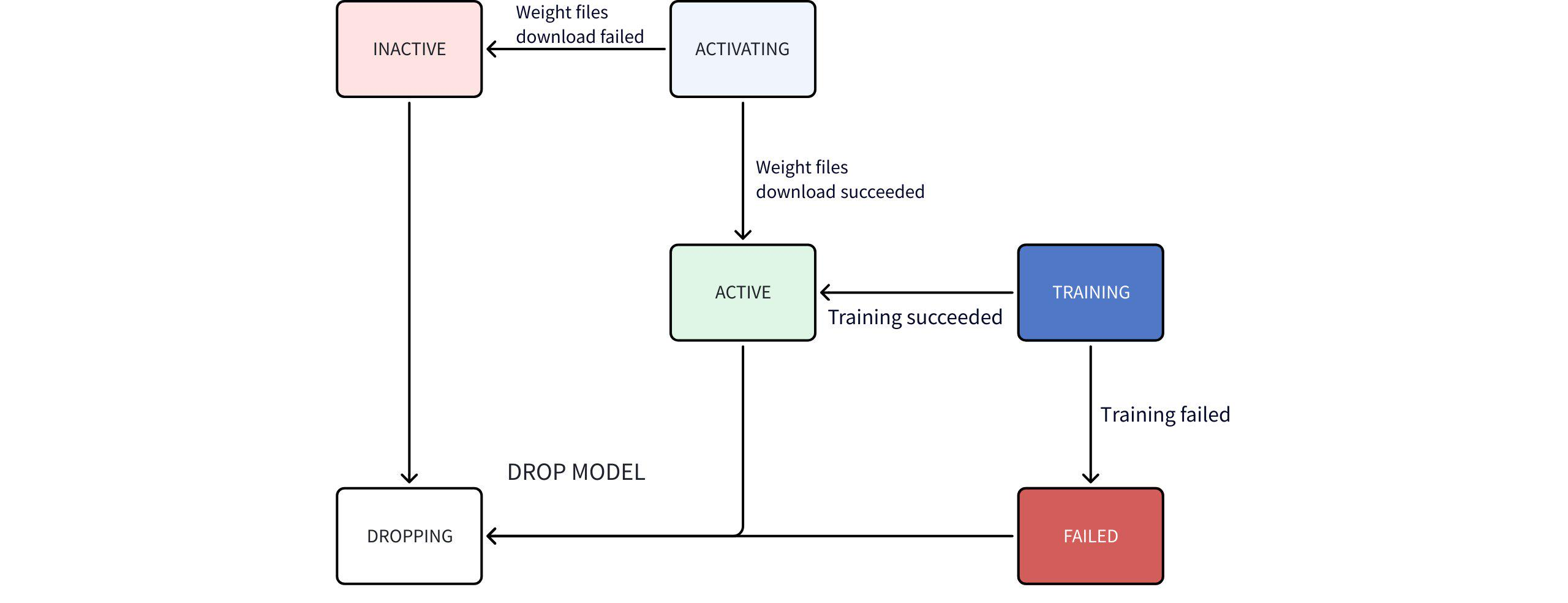
State machine flow description:
- After starting AINode, executing
show modelscommand, only system built-in (BUILTIN) models can be viewed. - Users can import their own models, which are identified as user-defined (USER_DEFINED); AINode will try to parse the model type (ModelType) from the model configuration file; if parsing fails, this field will be displayed as empty.
- Time series large models (built-in models) do not have weight files packaged with AINode, and AINode automatically downloads them when starting.
- During download, it is ACTIVATING, and after successful download, it becomes ACTIVE, and if failed, it becomes INACTIVE.
- After users start a model fine-tuning task, the model state during training is TRAINING, and after successful training, it becomes ACTIVE, and if failed, it becomes FAILED.
- If the fine-tuning task is successful, after fine-tuning, all ckpt (training files) will be statistically analyzed to find the best file and automatically renamed to the user-specified model_id.
Viewing Example
IoTDB> show models
+---------------------+--------------+--------------+-------------+
|              ModelId|     ModelType|      Category|        State|
+---------------------+--------------+--------------+-------------+
|                arima|        sktime|       builtin|       active|
|          holtwinters|        sktime|       builtin|       active|
|exponential_smoothing|        sktime|       builtin|       active|
|     naive_forecaster|        sktime|       builtin|       active|
|       stl_forecaster|        sktime|       builtin|       active|
|         gaussian_hmm|        sktime|       builtin|       active|
|              gmm_hmm|        sktime|       builtin|       active|
|                stray|        sktime|       builtin|       active|
|               custom|              |  user_defined|       active|
|             timer_xl|         timer|       builtin|   activating|
|              sundial|       sundial|       builtin|       active|
|           sundialx_1|       sundial|    fine_tuned|       active|
|           sundialx_4|       sundial|    fine_tuned|     training|
|           sundialx_5|       sundial|    fine_tuned|       failed|
|             chronos2|            t5|       builtin|     inactive|
+---------------------+--------------+--------------+-------------+
Built-in Traditional Time Series Models:
| Model Name | Core Concept | Applicable Scenarios | Key Features |
|---|---|---|---|
| ARIMA (Autoregressive Integrated Moving Average) | Combines AR, differencing (I), and MA for stationary or differenced series | Univariate forecasting (stock prices, sales, economics) | 1. For linear trends with weak seasonality2. Requires (p,d,q) tuning3. Sensitive to missing values |
| Holt-Winters (Triple Exponential Smoothing) | Exponential smoothing with level, trend, and seasonal components | Data with clear trend & seasonality (monthly sales, power demand) | 1. Handles additive/multiplicative seasonality2. Weights recent data higher3. Simple implementation |
| Exponential Smoothing | Weighted average of history with exponentially decaying weights | Trending but non-seasonal data (short-term demand) | 1. Few parameters, simple computation2. Suitable for stable/slow-changing series3. Extensible to double/triple smoothing |
| Naive Forecaster | Uses last observation as next prediction (simplest baseline) | Benchmarking or data with no clear pattern | 1. No training needed2. Sensitive to sudden changes3. Seasonal variant uses prior season value |
| STL Forecaster | Decomposes series into trend, seasonal, residual; forecasts components | Complex seasonality/trends (climate, traffic) | 1. Handles non-fixed seasonality2. Robust to outliers3. Components can use other models |
| Gaussian HMM | Hidden states generate observations; each state follows Gaussian distribution | State sequence prediction/classification (speech, finance) | 1. Models temporal state transitions2. Observations independent per state3. Requires state count |
| GMM HMM | Extends Gaussian HMM; each state uses Gaussian Mixture Model | Multi-modal observation scenarios (motion recognition, biosignals) | 1. More flexible than single Gaussian2. Higher complexity3. Requires GMM component count |
| STRAY (Search for Outliers using Random Projection and Adaptive Thresholding) | Uses SVD to detect anomalies in high-dimensional time series | High-dimensional anomaly detection (sensor networks, IT monitoring) | 1. No distribution assumption2. Handles high dimensions3. Sensitive to global anomalies |
Built-in Time Series Large Models:
| Model Name | Core Concept | Applicable Scenarios | Key Features |
|---|---|---|---|
| Timer-XL | Long-context time series large model pretrained on massive industrial data | Complex industrial forecasting requiring ultra-long history (energy, aerospace, transport) | 1. Supports input of tens of thousands of time points2. Covers non-stationary, multivariate, and covariate scenarios3. Pretrained on trillion-scale high-quality industrial IoT data |
| Timer-Sundial | Generative foundation model with "Transformer + TimeFlow" architecture | Zero-shot forecasting requiring uncertainty quantification (finance, supply chain, renewable energy) | 1. Strong zero-shot generalization; supports point & probabilistic forecasting2. Flexible analysis of any prediction distribution statistic3. Innovative flow-matching architecture for efficient non-deterministic sample generation |
| Chronos-2 | Universal time series foundation model based on discrete tokenization | Rapid zero-shot univariate forecasting; scenarios enhanced by covariates (promotions, weather) | 1. Powerful zero-shot probabilistic forecasting2. Unified multi-variable & covariate modeling (strict input requirements): a. Future covariate names ⊆ historical covariate names b. Each historical covariate length = target length c. Each future covariate length = prediction length3. Efficient encoder-only structure balancing performance and speed |
4.5 Model Deletion
Registered models can be deleted via SQL. AINode removes the corresponding model folder under user_defined. Syntax:
DROP MODEL <model_id>- Requires specifying an existing
model_id. - Deletion is asynchronous (status:
DROPPING), during which the model cannot be used for inference. - Built-in models cannot be deleted.
4.6 Loading/Unloading Models
AINode supports two loading strategies:
- On-Demand Loading: Load model temporarily during inference, then release resources. Suitable for testing or low-load scenarios.
- Persistent Loading: Keep model instances resident in CPU memory or GPU VRAM to support high-concurrency inference. Users specify load/unload targets via SQL; AINode auto-manages instance counts. Current loaded status is queryable.
Details below:
Configuration Parameters
Edit these settings to control persistent loading behavior:# Ratio of total device memory/VRAM usable by AINode for inference # Datatype: Float ain_inference_memory_usage_ratio=0.4 # Memory overhead ratio per loaded model instance (model_size * this_value) # Datatype: Float ain_inference_extra_memory_ratio=1.2List Available Devices
SHOW AI_DEVICESExample:
IoTDB> SHOW AI_DEVICES
+-------------+
|     DeviceId|
+-------------+
|          cpu|
|            0|
|            1|
+-------------+
Load Model
Manually load model; system auto-balances instance count based on resources:LOAD MODEL <existing_model_id> TO DEVICES <device_id>(, <device_id>)*Parameters:
existing_model_id: Model ID (current version supportstimer_xlandsundialonly)device_id:cpu: Load into server memorygpu_id: Load into specified GPU(s), e.g.,'0,1'for GPUs 0 and 1
Example:
LOAD MODEL sundial TO DEVICES 'cpu,0,1'Unload Model
Unload all instances of a model; system reallocates freed resources:UNLOAD MODEL <existing_model_id> FROM DEVICES <device_id>(, <device_id>)*Parameters same as
LOAD MODEL.
Example:UNLOAD MODEL sundial FROM DEVICES 'cpu,0,1'View Loaded Models
SHOW LOADED MODELS
SHOW LOADED MODELS <device_id>(, <device_id>)*  -- Filter by device
Example (sundial loaded on CPU, GPU 0, GPU 1):
IoTDB> SHOW LOADED MODELS +-------------+--------------+------------------+ | DeviceId| ModelId| Count(instances)| +-------------+--------------+------------------+ | cpu| sundial| 4| | 0| sundial| 6| | 1| sundial| 6| +-------------+--------------+------------------+DeviceId: Device identifierModelId: Loaded model IDCount(instances): Number of model instances per device (auto-assigned by system)
4.7 Large Time Series Models
AINode supports multiple large time series models. For deployment details, refer to Time Series Large Model
5. Permission Management
Use IoTDB's built-in authentication for AINode permissions. Users need USE_MODEL permission to manage models and access input data for inference.
| Permission | Scope | Administrator (default ROOT) | Normal User |
|---|---|---|---|
| USE_MODEL | create model / show models / drop model | √ | √ |
| READ_SCHEMA&READ_DATA | forecast | √ | √ |