
Basic Concepts
Basic Concepts
1. Common Concepts in Time-Series Databases
This section introduces common basic concepts in the time-series database field, including time-series data, time series, devices, timeseries, data points, sampling frequency, TTL, metadata, encoding, and compression.
1.1 Time-Series Data
In scenarios such as IoT, industrial production, energy and power, connected vehicles, and infrastructure monitoring, devices usually use sensors to continuously collect status data about themselves or their environment. For example, a motor collects voltage and current, a wind turbine collects blade rotation speed, angular velocity, and generated power, a vehicle collects longitude, latitude, speed, and fuel consumption, and a bridge collects vibration frequency, deflection, and displacement.
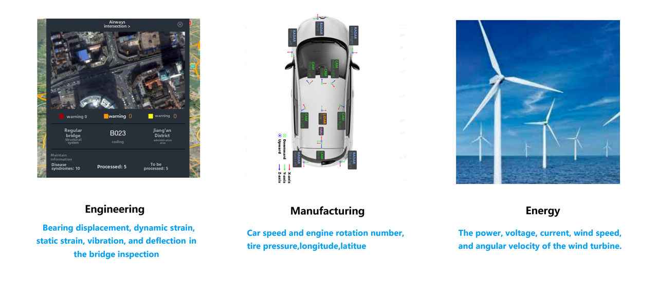
The common feature of this type of data is that it is time-related: the same collection object continuously produces new records as time passes. Data that is continuously produced and recorded in chronological order is called time-series data.
1.2 Time Series
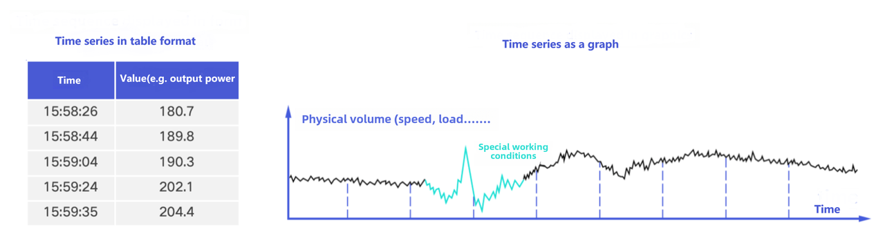
In time-series data scenarios, a collection point continuously produces data points over time. After these data points are arranged in ascending timestamp order, they form a time series. In tabular form, a time series can be represented as a data table composed of time and value. In graphical form, a time series can be represented as a trend curve that changes over time. It can also be described figuratively as a device's "electrocardiogram".
1.3 Device
A device, also called an entity or equipment, is a device or apparatus that has physical quantities in a real-world scenario. It can be a physical device, a measurement apparatus, or a set of sensors.
Common examples are as follows:
| Scenario | Device Example | Identifier Example |
|---|---|---|
| Energy | Wind turbine | Region, station, line, model, instance, etc. |
| Factory | Robotic arm | Unique ID generated by an IoT platform |
| Connected vehicle | Vehicle | Vehicle Identification Number (VIN) |
| Monitoring | CPU | Machine room, rack, hostname, device type, etc. |
1.4 Timeseries / Field
A timeseries can also be called a physical quantity, time series, timeline, signal, metric, point, or measured value. It is measurement information recorded by a detection device in a real-world scenario. Usually, a physical quantity represents a collection point that can periodically collect the physical quantity of the environment or device where it is located. When the data points generated by a timeseries over time are arranged in ascending timestamp order, they form a time series.
Common examples are as follows:
| Scenario | Timeseries Example |
|---|---|
| Energy and power | Current, voltage, wind speed, rotation speed |
| Connected vehicle | Fuel level, vehicle speed, longitude, latitude |
| Factory | Temperature, humidity |
In the IoTDB table model, the number of timeseries equals the sum of the timeseries counts across all tables. The number of timeseries in each table equals the number of devices multiplied by the number of field columns. For the detailed counting method, see Metadata Query.
1.5 Data Point
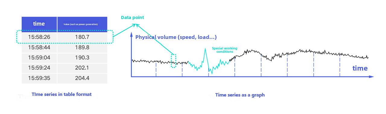
A data point consists of a timestamp and a value. The timestamp indicates when the data was generated, and the value indicates the collection result of the timeseries at that time. The value can be of multiple types, such as BOOLEAN, FLOAT, and INT32.
A row in a tabular time series, or a point in a trend chart, can both be understood as a data point.
1.6 Sampling Frequency
Sampling frequency refers to the number of times a physical quantity generates data within a certain period of time. For example, if a temperature sensor collects temperature data once per second, the sampling frequency is 1 Hz, that is, once per second.
The higher the sampling frequency, the more data points are generated per unit of time, and the higher the requirements for writing, storage, and query capabilities.
1.7 Data Retention Time (TTL)
TTL is used to specify the data retention time. Data beyond the TTL will be automatically deleted.
Using TTL properly can control disk space usage, avoid issues such as disks becoming full, and help maintain query performance and reduce memory resource usage.
1.8 Metadata (Schema)
Metadata is the data model information of a database and is used to describe the structure and definition of data. For time-series data, metadata usually includes information such as devices, timeseries, and data types.
1.9 Encoding and Compression
Encoding is a compression technique used to represent data in binary form, thereby improving storage efficiency. Compression further compresses binary data after encoding to improve storage efficiency.
For details about the encoding and compression methods supported by IoTDB, see Compression and Encoding.
2. Common IoTDB Concepts
This section introduces common concepts in IoTDB data models, distributed architecture, and deployment. These concepts explain how IoTDB organizes, manages, and deploys time-series data.
2.1 Data Model Concepts
2.1.1 Data Model (sql_dialect)
IoTDB supports two data models: the tree model and the table model. Both models manage devices and timeseries as their core objects, but they organize data differently and use different syntax.
Tree model: Manages data by using hierarchical paths. One path corresponds to one timeseries of one device.
Table model: Manages data by using relational tables. One table is recommended to correspond to one type of device.
Two model spaces can exist in the same cluster instance. Different models use different syntax and database naming methods, and are not visible to each other by default.
2.1.2 Database
In the table model, a database is an upper-level organizational structure that can manage multiple types of devices and their tables. Before creating tables, writing data, or querying data, you usually need to create a database first.
2.1.3 Table
In the table model, it is recommended that one table correspond to one type of device during modeling, and the table is used to organize the time-series data of that type of device. Devices of the same type usually have the same or similar sets of timeseries.
2.1.4 Time Column, Tag Column, Attribute Column, and Field Column
Columns in the table model can be divided by purpose into time columns, tag columns, attribute columns, and field columns.
| Concept | Description |
|---|---|
| Time column (TIME) | Each table must contain one time column, whose data type is TIMESTAMP |
| Tag column (TAG) | Used to identify devices and can act as a composite primary key for devices. It usually does not change over time |
| Attribute column (ATTRIBUTE) | Used to describe static attributes of devices. It does not change over time and can be updated or added |
| Field column (FIELD) | Used to store timeseries values collected by devices. Values change over time |
In terms of data filtering efficiency, this can usually be understood as: time columns and tag columns take priority, followed by attribute columns, and then field columns.
2.2 Distributed Concepts
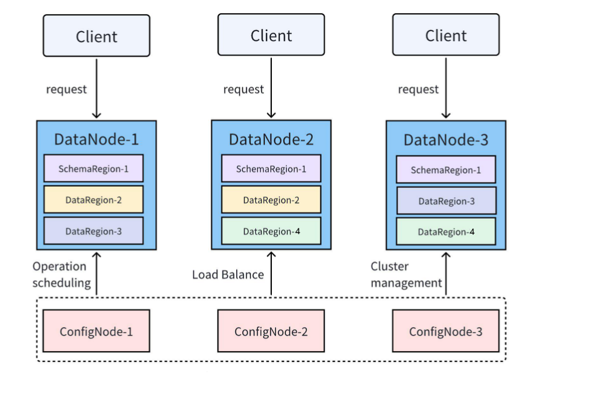
IoTDB supports running in cluster mode. Common concepts in a cluster include nodes, Regions, and multiple replicas. A common cluster deployment pattern is 3C3D, that is, 3 ConfigNodes and 3 DataNodes.
2.2.1 Node
An IoTDB cluster includes three types of nodes: ConfigNode, DataNode, and AINode.
ConfigNode: Manages cluster node information, configuration information, user permissions, metadata, partition information, and more. It is responsible for scheduling distributed operations and load balancing. All ConfigNodes are full backups of each other.
DataNode: Serves client requests and is responsible for data storage and computation.
AINode: Provides machine learning capabilities, supports registering trained machine learning models, and invokes models for inference through SQL.
2.2.2 Data Partition (Region)
In IoTDB, metadata and data are divided into smaller partitions, called Regions, and are managed by DataNodes in the cluster.
SchemaRegion: A metadata partition used to manage the metadata of some devices and timeseries.
DataRegion: A data partition used to manage the data of some devices within a time range.
Regions with the same RegionID on different DataNodes are replicas of each other.
2.2.3 Multiple Replicas
The number of replicas for data and metadata is configurable. Multiple replicas can provide high availability.
| Category | Configuration Item | Recommended Standalone Configuration | Recommended Cluster Configuration |
|---|---|---|---|
| Metadata | schema_replication_factor | 1 | 3 |
| Data | data_replication_factor | 1 | 2 |
2.3 Deployment Concepts
IoTDB has three running modes: standalone mode, cluster mode, and dual-active mode.
2.3.1 Standalone Mode
An IoTDB standalone instance includes 1 ConfigNode and 1 DataNode, that is, 1C1D.
Feature: Easy for developers to install and deploy, with low deployment and maintenance costs and convenient operations.
Applicable scenarios: Scenarios with limited resources or low high-availability requirements, such as edge servers.
Deployment method: Standalone Deployment
2.3.2 Dual-Active Mode
Dual-active deployment is a feature of TimechoDB. It means two independent instances synchronize with each other bidirectionally and can provide services externally at the same time. After one instance stops and restarts, the other instance resumes transferring the missing data from the breakpoint.
An IoTDB dual-active instance usually consists of two standalone nodes, that is, two sets of 1C1D. Each instance can also be a cluster.
Feature: A high-availability solution with the lowest resource usage.
Applicable scenarios: Scenarios with limited resources (only two servers) but a need for high availability.
Deployment method: Dual-Active Deployment
2.3.3 Cluster Mode
An IoTDB cluster instance has 3 ConfigNodes and no fewer than 3 DataNodes, usually 3 DataNodes, that is, 3C3D. When some nodes fail, the remaining nodes can still provide services externally, ensuring high availability of database services. Database performance can also be improved as nodes are added.
Feature: High availability and high scalability. System performance can be improved by adding DataNodes.
Applicable scenarios: Enterprise-level application scenarios that require high availability and reliability.
Deployment method: Cluster Deployment
2.3.4 Feature Summary
| Dimension | Standalone Mode | Dual-Active Mode | Cluster Mode |
|---|---|---|---|
| Applicable scenarios | Edge deployment and scenarios with low high-availability requirements | High-availability services, disaster recovery scenarios, etc. | High-availability services, disaster recovery scenarios, etc. |
| Number of required machines | 1 | 2 | >=3 |
| Safety and reliability | Cannot tolerate a single point of failure | High, can tolerate a single point of failure | High, can tolerate a single point of failure |
| Scalability | DataNodes can be expanded to improve performance | Each instance can be expanded as needed | DataNodes can be expanded to improve performance |
| Performance | Can scale with the number of DataNodes | Same as one of the instances | Can scale with the number of DataNodes |
- The deployment steps for standalone mode and cluster mode are similar (ConfigNodes and DataNodes are added one by one). The only differences are the number of replicas and the minimum number of nodes that can provide services.